
Pre-Investment Considerations
Diving Deeper Into Assessing Future Greenhouse Gas Impact

It is amazing to witness the growth of the field of impact accountability since Prime Coalition and NYSERDA’s first Emissions Reduction Potential (ERP) methodology in late 2017. As the need for meaningful climate solutions becomes all the more pressing, Galvanize is energized by the efforts of the Project Frame community to ensure our sector’s collective investments yield the greatest climate benefit, and we look forward to learning from their evolving guidance.
Nicole Systrom, Chief Impact Officer, Galvanize Climate Solutions
Table of Contents
1.1 Qualifying Impact and Effects
1.3 Defining and Quantifying Units
1.4 Obtaining Emissions Factors
1.5 Constructing the Baseline Scenario
Section 2: Potential GHG Impact
2.3 The S-Curve: Market Adoption and Technology Diffusion
2.4 Calculating Potential Impact
3.2 Calculating Planned Impact
Project Frame is not a regulatory body, nor should its content be considered financial advice. Methodology guidance produced by Project Frame represents our contributors’ consensus and no one singular entity. Our work is intended for readers to review and use their best judgement to accelerate GHG mitigation with transparency and accountability.

As practitioners, it is critical for us to develop common practices to assess the forward-looking emissions impact of emerging climate solutions. Although difficult, alignment on these assessment methodologies, developed through collaborations such as those fostered by Project Frame, will be the catalyst to unlock the trillions in capital needed and measure the impact to address the climate crisis.
Neil Yeoh, CEO, OnePointFive
Foreword
We are pleased to introduce the latest and most significant Project Frame methodology guidance, Diving Deeper into Assessing Greenhouse Gas Impact.
During the past few years, we have seen large increases in capital allocated to green technologies and reduction of greenhouse gas (GHG) emissions into the atmosphere has become a key metric to track the performance of companies, funds, and fund managers. Reporting on estimated GHG emissions is becoming nearly universal — and may soon become mandatory — for most mature businesses and financial enterprises. This reporting is governed by the World Resources Institute/World Business Council for Sustainable Development (WRI/WBCSD) GHG Protocol. However, when it comes to estimating expected future GHG savings, there are no common standards. We sometimes see companies and investors compete to report the highest impact numbers from their projects or investments, perhaps encouraged by financial incentives linked to these numbers. It is only through the most accurate reporting possible can we serve the ultimate purpose of allocating capital to investments with the highest real impact.
The ambition of Project Frame is to build consensus around common impact terminology and best practices and thereby better direct climate-focused investment toward highest-potential solutions. This methodology is a collaboration among dozens of respected climate
investors. Through these efforts, we hope to build a global community of investors that work collaboratively to improve reporting quality and transparency.
Measuring impact is a challenging task, but this should not discourage us from making progress one step at a time. While the endeavor must always take into account unique circumstances, and will never be perfectly accurate, achieving greater commonality in practices like setting baselines can improve the comparability and transparency of impact measurement. We see this methodology as a starting point for more research and collaboration among Frame members, scientists, and other experts and practitioners.
We have been privileged to serve on Frame’s Steering Committee (SC) alongside other distinguished members. We appreciate the leadership provided by Prime Coalition, Project Frame Director Keri Browder, and our fellow SC members. In a world that is increasingly fragmented in many areas and facing greater urgency for climate action, Frame is an important contribution to fostering both international cooperation and climate change mitigation
Peter Fox-Penner
Chief Impact Officer, Energy Impact Partners
Siri Kalvig
Chief Executive Officer, Nysnø Climate Investments

Economic data alone cannot reveal the full return potential of any given investment. As climate impact becomes increasingly acknowledged as a value driver and leading indicator for investors, a common language and shared measurement and management instruments are needed to accelerate change and promote accountability. With this methodology, Project Frame lays the important groundwork in this fast-emerging field, enabling climate investors and ventures to collaborate on impactful decarbonization solutions.
Daniel Valenzuela, Head of IR & Impact, World Fund
Welcome
We all have a role to play to ensure a livable climate.
Project Frame (Frame) brings together investors as well as climate and impact experts to build common terminology, methodology, and best practices to accelerate the flow of capital to the best possible climate solutions while prioritizing transparency and accountability. This paper builds on the work Project Frame released in early 2022, beginning with our guiding principles and our previous paper, An Introduction to Assessing Planned Greenhouse Gas (GHG) Impact. Frame’s intention is to build consensus around best practices for venture capital and private equity climate investing while demystifying the field in order to drive more capital towards solutions for a liveable climate. Every resource allocation decision we make will have ripple effects. In this paper, we focus solely on creating a high-level methodology for screening investments based on GHG impact. In the future, we hope to dive deeper into sectors, mitigating unintended social and environmental consequences, and solutions themselves.
This iteration of our pre-investment guidance consolidates the expertise of eight original authors, ten internal reviewers and contributors, as well as outside reviewers and 30 focus group members from leading climate investing firms; it’s the second of many future iterations. We hope that venture and private equity investors will adapt our guidance to their practices and provide feedback to inform our continued efforts as we consider engaging other asset classes.
This iteration of our evolving methodology is dedicated to untangling the complexities of assessing forward-looking GHG impact pre-investment, or the impact an investment could have in mitigating emissions. This is distinct from footprinting, which is largely focused on reconciling an individual or organization’s overall emissions. This is also distinct from life cycle analysis (LCA), though LCA can often be an important factor when assessing forward-looking impact. We explain the relationship between LCA and our methodology later in this paper.
Forward-looking GHG impact assessments are an evolving practice, but we are proud of the progress our working group has made to reach consensus on several aspects of pre-investment emissions impact screening and to highlight areas that require further debate. We look forward to diving deeper in the months and years ahead. You may find that not every topic applies to your practice. Topics have been grouped into chapters for easier navigation, which we hope will allow you to focus on those that best serve your needs throughout your climate investing journey.
While reading the paper, it is important to note when examples describe a solution versus a company. Generally speaking, most investors assess a company prior to investment. For our purposes, we often analyze the potential or planned emissions of a proposed climate solution, the definition of which you can find, among other useful terms for orientation, in our glossary. Reaching consensus around the use of terminology within the climate investing space is a consistent challenge that we enjoy tackling alongside the industry leaders who make up the Project Frame community.
It is also important to mention that the Content Working Group was not always able to reach 100% consensus on aspects of the methodology. In order to move the methodology forward, we convened a focus group alongside our working group members to vote on areas where we struggled to reach alignment. In particular, we sought guidance on the Impact Type and Attribution sections. For Impact Type, 80% of the focus group agreed with our terminology for qualification and 87% with our quantification recommendations. For the latter section, it stood out to us that only 40% of respondents said that attribution was a factor for pre-investment screening or post investment reporting. Bearing this in mind, 90% agreed with our recommendations for horizontal attribution, whereas 70% agreed with the recommendations for vertical. In Frame, we often say “this is an evolving practice” or a snapshot of a moment in time, and we will continue to revise recommendations based on consensus for future iterations.
We are not a prescriptive body, but we are encouraged by the feedback we received from our focus group indicating an interest in aligning their investment practices with the recommendations proposed by Project Frame (consistently over 85%, across several categories). We do not take this responsibility lightly and look forward to growing together. Frame’s aim is to enable seamless and efficient communications between entrepreneurs and investors so that we can all spend more time and energy delivering impact.

Investing in climate solutions requires an analytical and science-based approach to calculating net impact over time. AENU is proud to use Project Frame’s methodology for assessing and tracking potential, planned, and next, realized GHG reductions impact, for both new investment opportunities and our own portfolio.
Melina Sánchez Montañés, Principal & VP Impact, AENU
How To Navigate
Before diving into the background and steps for the methodology in detail, it's important to understand that Frame differentiates two overarching methodologies for assessing “impact.”
Project Frame defines impact as the way a solution is expected to directly or indirectly result in a change in Greenhouse Gas (GHG) emissions when compared to a defined status quo or incumbent.
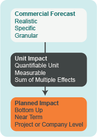
Potential impact is based on what the solution could achieve, assuming a standardized trajectory of success. Potential impact is calculated top-down based on TAM, SAM, and relevant diffusion or S-curves.
Planned impact is based on what the company deploying the solution intends to achieve per a realistic analysis of its business model. Planned impact from companies is a bottom-up approach based on the specific business plan and sales forecast for the company, accounting for their current resources, offerings, and capabilities.
The difference between potential and planned impact lies in how the calculations account for a future deployment of the solution.

All of the impact assessments utilize a common unit impact calculation approach. The forward-looking impact of a proposed climate solution is the impact of a single unit times the number of units deployed (Equation 1). A unit is an instance that quantifies an amount of product or service, which is used to compare a solution to an incumbent. Therefore, the unit impact can be expressed as the difference in emissions between one unit of the incumbent and one unit of the solution. For further orientation to Frame’s terminology, please reference the Project Frame glossary on our website.
Whether you use planned or potential impact will be decided by your investment and/or impact teams. However, Section 1: Unit Impact is a prerequisite for either. If you are newer to forward-looking impact, we suggest starting with Section 2: Potential GHG Impact and working towards Section 3: Planned GHG Impact analysis. Projections using the potential impact approach are optimal for assessing a broader class of technologies or solutions and are more hypothetical in nature. Projections using the planned impact approach are more concrete and are therefore best for assessing a specific company, project, or portfolio, where specific business plans and sales forecasts are available. In Section 4, we discuss other important considerations: attribution and additionality. While these concepts aren’t necessarily common practice for all climate investors, we feel they are worth covering as important aspects of many investors' pre-investment screening process.
Among Project Frame's principles are transparency and conservatism; as a best practice, Frame recommends indicating your selected approach in your reporting and taking care to avoid overestimating GHG values.
How Unit Impact Supports the Calculation of Potential or Planned Impact


Section 1
Unit Impact
In this section, we describe how to tell the story of a potential climate solution and how to calculate its unit impact, the most essential building block of potential or planned impact analysis. This impact quantification works best for solutions that are relatively standardized goods or service bundles in multiple quantities where it is easy to analyze impacts on a per-unit basis.
In its simplest form, the forward-looking impact of a proposed climate solution is the impact of a single unit times the
number of units deployed. A unit is an instance that quantifies an amount of product or service, which is used to compare a solution to an incumbent.
Therefore, unit impact can be expressed as the difference in emissions between one unit of the incumbent and one unit of the solution. It is important to note that unit impact is not a constant: Emissions from both the incumbent and the solution may change over time.
1.1
Qualifying Impact and Effects
1.1.1 The Impact Story
Everything starts with a story: The potential or planned impact of a proposed climate solution needs first to be described in relatable terms. The impact of a solution is often the result of several overlapping effects that lead, eventually, to the reduction of the GHG emissions. Our methodology endeavors to give more details to the numbers being calculated, so that the reader or the analyst can relate to these figures in a reliable manner.
Articulating the proposed impact of an overall solution is commonplace among climate investors; however, the language and the level of detail varies widely. We hope that the language provided, which was largely influenced by the practices of Project Frame members and feedback from our focus group, will help us build consensus and consistency for future assessments and reporting.
Our methodology defines a segmentation of the solution in different categories and then proposes a systematic approach to identify and characterize all the effects that a solution generates.

Qualification of the solution
1.1.2 Characterize the Scope of Solution
GHG impact is rarely the result of only one solution. This second criteria aims to describe what type of contribution a solution has in the overall chain of contributors.
-
When a solution can be purchased as a whole to yield GHG impact (for example, an electric vehicle, heat pump, or more sustainably produced food product).
-
A part of an overall solution that plays a critical role in delivering GHG impact. The GHG impact will depend on the use case for the product that contains the component (for example, an EV battery, lighter materials, a more efficient motor, recycled materials within a product, or an efficiency upgrade) .
-
Often also referred to as an ‘enabling’ solution. A solution that advances our ability to reduce emissions or adopt an emerging solution that ultimately delivers or accelerates GHG impact (for example, trading platforms, advocacy campaigns, methane leak detection, software, process improvements, or devices that improve consumer awareness).
Just being a component or process associated with a product doesn’t automatically qualify as a climate solution. For example, the tires of an electric vehicle do not qualify if they are made out of the same materials as regular ICE vehicles. New roads wouldn’t be a component unless they were made with advanced materials or processes to reduce GHG emissions. However, a new highway that reduced traffic congestion and improved the effective mileage of vehicles using it could be considered as a “facilitating” solution.
1.1.3 List and Qualify the Solution’s Generated Effects
A solution often generates multiple effects that may or may not be linked to one another. The impact storyteller needs to describe each of these effects separately.
| Description | Reducing/Increasing | Recurrence of Effect | How is it measured? | |
|---|---|---|---|---|
| Effect A | (...) | (...) | (...) | (...) |
| Effect B | (...) | (...) | (...) | (...) |
| Effect C | (...) | (...) | (...) | (...) |
Listing and Qualification of the Effects
-
Describe each effect of the solution in relatable terms. This exercise should help articulate the different mechanisms through which the GHG impact is generated (in some cases, consider whether or not the solution will impact supply or demand).
-
Define whether the given effect contributes to reducing or increasing the overall GHG emissions; examples of an increasing contribution could be a rebound effect or embedded emissions at the manufacturing stage.
-
Qualify how the effect lasts over time.
One-off: Effects produced once over the lifetime of the product (i.e., plant-based meat substitute)
Recurring: Effects produced repeatedly, often over a period of time and typically the operating lifetime of the solution. Through this criteria, we are borrowing from finance and accounting terminology, where recurring and one-off revenues are used. (i.e., a photovoltaic (PV) panel that will produce low carbon power over 30 years). Recurring effects may also be called “fleet effects” because they depend not on products sold but on the size of the fleet in operation. Fleet effect is discussed in more detail in Section 2.4.1.
-
Present how the given effect will be quantified and monitored over time:
Measured directly
Inferred from other measurements
Estimated using models
Not quantified due to lack of data or because it’s non-significant
Some effects of a given solution may be identified but ultimately excluded from a quantitative forward-looking impact analysis, particularly if they are expected to be orders of magnitude lower than the more significant effects. Take, for instance, a solution related to lithium-ion (Li-ion) batteries. Energy and material requirements for batteries produce emissions, but the solution also reduces emissions by enabling EVs and renewables. The analyst may decide not to study the embedded emissions of the battery because they assume that it is dwarfed by the emissions-reducing effect of displacing fossil energy. Making and documenting assumptions of this type can dramatically accelerate the analysis process, simplify the analysis itself, and leave room for model refinement in the future or by third parties.
In the example in Table 3, taken from a real investment, the solution is a new material that allows the battery from an EV to be 10% lighter in mass.
| Description | Reducing/Increasing | Recurrence of Effect | How is it measured? | |
|---|---|---|---|---|
| Effect A | The car equipped with the battery will use 3% less energy for the same number of km | Reduce | Recurring The effect will be produced over the lifetime of the battery |
Estimated |
| Effect B | The battery needs 25 kg of copper and 50 kg of lithium to be produced, as well as 150 kWh of power more than standard battery | Increase | One-off
This effect only occurs once, at manufacturing stage |
Measured |
| Effect C | The lighter battery improves the features of the EV and contributes to enticing the shift from an ICE car to EV at the time of purchase, making the product more appealing than the ICE vehicle | Reduce | One-off This effect materializes at the same time of purchase |
Not quantifiable |
Table 3: Example list of effects for a solution consisting of producing a battery 10% lighter for the EV market (additional examples can be found in the appendix).
For every effect that can be quantified (either measured, inferred, or estimated), the unit impact of that effect can be calculated using Equation 1. Because the quantities in this equation are not constant, we recommend that unit impact be calculated for each year i in the forward-looking analysis.
Unit Impactᵢₑ = Incumbent Unit Emissionsᵢₑ
- Solution Unit Emissionsᵢₑ
+ Solution Unit GHG Removalᵢₑ
Equation 1: Unit impact for effect e in year i
1.1.4 Consider GWP and GHG Type
“Global Warming Potential” (GWP) consists of multipliers applied to greenhouse gasses such as methane (CH₄) and nitrous oxide (N₂O) to equate the impact they have on the Earth’s temperature with that of carbon dioxide (CO₂) over a particular time horizon. It provides a common scale for measuring the climate effects of different gasses.
According to guidance from the GHG Protocol and AR6 of the Intergovernmental Panel on Climate Change (IPCC), to account for warming and lifetime differences, the GWP of a GHG for a particular time frame is used (usually 100 years (GWP100) or 20 years (GWP20)). Since GWP is defined as warming relative to CO₂, the GWP of CO₂ is 1 for any timeframe. The GWP20 of fossil-origin methane is 82.5, and the GWP100 of fossil-origin methane is about 29.8. In other words, a ton of methane emissions is considered to have about 29.8 times the warming of CO₂ over a 100-year time horizon.
The reason for the GWP difference between fossil-origin and non-fossil-origin methane is that methane degrades to CO₂ over time, and the CO₂ from fossil-origin is newly introduced to the atmosphere, while CO₂ from non-fossil-origin methane (e.g., from cows) came out of the atmosphere recently, when the methane was created.
| Greenhouse Gas | GWP-20 | GWP-100 | GWP-500 |
|---|---|---|---|
| Carbon Dioxide (CO2) | 1 | 1 | 1 |
| Methan fossil origin (CH4) | 82.5 | 29.8 | 10 |
| Methane non-fossil origin (CH4) | 79.7 | 27 | 7.2 |
| Nitrous Oxide (N2O) | 273 | 273 | 130 |
Carbon Dioxide vs. Methane Emissions: What’s the difference?
After carbon dioxide (CO₂) is emitted to the atmosphere, some portion of it is absorbed by the oceans, plants, and soils. The remaining amount stays in the atmosphere for hundreds to thousands of years, causing continued warming even if additional CO₂ emissions cease. Methane is a much more potent greenhouse gas and is about 120 times as effective at trapping heat compared to CO₂. However, methane (CH₄) breaks down in the atmosphere (to CO₂) after about 12 years, so its effective long-term warming potential is 82.5X over a 20-year horizon, or 29.8X over a 100-year horizon, compared to CO₂.
While the GHG Protocol and others use GWP100 for methane, using GWP20 is becoming more common as concern grows about the impacts of global warming over the next few decades. Evaluators should consider the short- and long-term impacts of proposed climate solutions; they should also carefully consider what time frames to use when assessing and reporting emissions, particularly methane. At a minimum, investors should align with the current IPCC guidance. With the intention of moving the field forward, Project Frame recommends that evaluators should run scenarios for shorting timescales, such as GWP20, and be clear and precise about any other GWP they are using in their analysis.
For more information about GWP, please visit GTI’s Center for Methane Research.
1.2
Setting System Boundaries
A proposed climate solution and its effects are informed by its relationship to a larger system. Project Frame defines a system boundary as the divide between what is included and what is excluded from a system of study.
The system boundary refers to the limits of the system or process being studied or evaluated, and it determines which activities and emissions sources are included or excluded. The "box is drawn" to highlight the extent to which GHG emissions are attributed to a particular product, process, organization, or sector. For example, the system boundary for a product may include emissions from its production, transportation, and use while excluding emissions from the production of inputs or disposal of waste. It is important to be transparent and consistent in defining the system boundary and to clearly communicate the scope and limitations of the emissions analysis to stakeholders.
Defining the system boundary is an essential step in calculating GHG emissions, as it affects the accuracy and completeness of the emissions inventory. Defining a system boundary too widely will be onerous for the analyst, and defining it too narrowly could result in a flawed analysis. Overly narrow system boundaries pose a risk of “greenwashing,” if the analyst sets the boundaries to include emissions reduction while excluding effects that increase emissions.
A well-thought-out set of system boundaries will result in a useful assessment that is not overly burdensome to produce. Project Frame recommends setting system boundaries wide enough to include all substantial effects of the proposed climate solution.
It is common to refer to “direct” or “indirect” emissions, otherwise known as Scope 1, 2, and 3 emissions. Scope 1, or direct, emissions are the result of a particular company's activities (running its factories, transporting its goods, etc.). Scope 2 and 3 emissions are indirect, meaning they are not emitted by the company but instead as a result of its actions: Scope 2 refers to the emissions from consumption of electricity and heat, and Scope 3 includes all other up- and downstream emissions (the emissions from the widgets that a company buys to make its gizmos, for example, and the emissions from the usage of those gizmos). One company’s indirect emissions are another’s direct emissions.
System boundaries may include all or some of the five lifecycle phases: raw material extraction, manufacturing, distribution, use, and disposal. For example, when comparing the unit impact of an electric vehicle (EV) displacing an internal combustion engine (ICE) vehicle as the incumbent, the system boundary should include emissions from fueling and maintaining the vehicles over their lifetime. It should also include emissions from materials and manufacturing of the vehicles.
To measure net impact, Equation 1 can be expanded to represent impact across each lifecycle phase. The model for unit impact for each effect can then be constructed, with the relevant quantities for incumbent and solution emissions expressed as an emissions factor (see Section 1.4).
Unit Impactᵢₑ = (Material emissions of incumbent - Material emissions of solution)ᵢₑ
+ (Manufacturing emissions of incumbent - Manufacturing emissions of solution)ᵢₑ
+ (Distribution emissions of incumbent - Distribution emissions of solution)ᵢₑ
+ (Use emissions of incumbent - Use emissions of solution)ie
+ (Solution carbon removal)ᵢₑ
+ (Disposal emissions of incumbent - Disposal emissions of solution)ᵢₑ
Equation 2: Unit impact for effect e in year i, expanded to include lifecycle phases
When reporting on the future impact of a solution, which displaces an incumbent relative to a counterfactual, analysts can omit any terms in Equation 2 that are outside the system boundary. Take, for example, a more efficient heat pump: It may be reasonable to assume that there is no significant change in emissions factors for material extraction, manufacturing, distribution, or disposal relative to a standard heat pump, in which case the system boundary would only include the use of the heat pump.
1.3
Defining and Quantifying Units
When evaluating potential climate solutions, there may be multiple options for defining the unit of production or consumption of the solution.
One product — for example, a single vehicle or a single solar panel.
One application of a product — for example, one MWh of electricity generated, one geothermal well drilled, or one vehicle mile traveled.
One plant producing a product — for example, one battery manufacturing facility or power generation facility.
One portion of a market — for example, a percentage of cargo shipping emissions that are captured.
Analysts must choose the solution unit to be comparable to the unit of the relevant incumbent (if there is one). For example, the availability of low-cost EVs could displace ICE vehicles as well as other modes of transportation, such as bicycles or public transportation. To account for this when assessing the forward-looking impact of an EV, the analyst would need to select a unit that is comparable across different modes of transportation, such as miles traveled. This would result in a more conservative estimate of impact, rather than assuming that EVs only displace high-emitting vehicles.
The proper choice of unit may be different for the various effects in a given solution, depending on the nature of the effect. Impact of a one-off effect that occurs during production, for example, is well-suited to “number of products sold” as the unit. The impact of a recurring “fleet effect” that occurs during use, however, may require “number of products operating” as the unit; see Section 2.4 for more on how this scenario affects the impact calculation.
The choice of unit can determine the simplicity — or complexity — of the calculations. Project Frame recommends choosing simpler calculations when all else is equal, for the sake of quality control, efficiency, and transparency. For example, if a solution involves point source carbon capture on ships, it may not be necessary to estimate the number of ships and average size of ship in order to arrive at future impact. If data are available on global cargo shipping emissions, the analyst can choose the unit to be the portion of cargo shipping in which the solution is deployed, which leads to a simpler calculation.
The choice of unit may also be influenced by the availability of data, for both the solution and the incumbent, as described below for emissions factors. Take, for example, an energy-efficient chemical production process for which the unit could be defined in terms of mass or volume. If data on the incumbent process are available as energy use per mass of material, then a wise choice for the unit of the solution might be one kilogram (kg) or one metric ton (MT).
1.4
Obtaining Emission Factors
Emissions factors relate the unit of the solution to an amount of pollutant emitted to the environment.
From Project Frame’s perspective, the pollutants of interest are GHGs. As such, emissions factors will typically be expressed in terms of kg CO₂e per unit of the solution being analyzed. Emissions factors often come from life cycle analysis or assessment (LCA), which is a cumulative accounting of all current measured GHG emissions connected to a particular product or process within a specified system boundary. LCAs may include Scopes 1, 2, and/or 3 emissions, as well as complex feedback loops, such as recycling processes.
Published LCAs and resulting emissions factors are useful resources for the forward-looking models we construct. LCA is also an academic field, with many practitioners and a codified methodology that has lessons for us to learn. However, the analyses can be difficult to interpret and, when used incorrectly, can lead to wildly erroneous calculations. While we are not attempting to train the reader in performing LCA, we hope in this section to provide clarity around how these analyses can be a resource for forward-looking GHG impact assessment. The end goal of reading an LCA is to find a reputable emissions factor for a product or process in the particular geography of interest.
Emissions factors may be straightforward to use, but they can also present interesting problems for the analyst. Take the example of grid emissions: per the EPA, the average emissions factor of the US grid in 2019 was 0.433 kg CO₂/kWh. However, if we had reduced electricity use by 1 kWh in 2019, we would have saved 0.709 kg CO₂. New generation or electricity generation displaces marginal electricity production, which depends heavily on time and place. Depending on the scale of the displaced or avoided energy usage, it may be more appropriate to use the average grid emissions factor rather than the marginal one.
Some LCAs are cradle-to-gate, meaning their system boundary stops at the output of a finished product, such as a car leaving the factory. Other LCAs are cradle-to-grave, meaning their system boundary includes the impact of the product at end of life. “Cradle” and “grave” are generally understood in absolute terms (i.e., materials originating from and returning to the environment, including waterways, soil/earth, and the atmosphere), whereas “gate” is a highly relative term and pathway specific.
Often, it is simple to find published emissions factors without parsing LCAs in detail, and yet it is important to check figures obtained from LCAs for believability, especially when the model has high sensitivity to the parameter in question.Even peer-reviewed and other high-quality white papers may contain order of magnitude mistakes due to simple unit conversion errors that are easy for anyone to miss. While every LCA has the same four components (see the appendix), their execution varies significantly, and any two LCAs of the same product or process may have drastically different outcomes. Poore and Nemecek provide a cautionary tale in their analysis of 1,530 LCAs, in which they find that 960 of them were unusable due to non-standard data reporting. The analyst should be sure to check their own work as well, avoiding notable pitfalls of dimensional analysis (see the appendix).
LCA standards use the term “impact” in a different way than Project Frame. While Project Frame always uses “impact” to compare one projected scenario to a counterfactual, LCAs typically refer to any calculated emissions, pollutants, energy usage, etc., from their defined scope as “impact.” The step in an LCA that produces emissions factors is called “Impact Assessment”; depending on the scope of the analysis, the emissions factor may refer to absolute quantity of emissions from a given activity, or the change in emissions relative to a counterfactual.
1.5
Constructing the Baseline Scenario
The concept of additionality described in Section 4.2 is closely tied to the evaluation of potential or planned GHG impact and, in fact, there usually is significant overlap between the two analyses. However, when determining potential or planned GHG impact, a baseline is used that may not be broad enough to account for all potential GHG flows or other, unconsidered factors that could affect GHG impact in a significant manner. An additionality analysis is an extra lens to view the potential climate solution to ensure that key factors that affect the net benefit of the proposed climate solution are considered. However, as is noted in Section 4.2, Project Frame has yet yo be able to reach consensus around the concept of “additionality” and will continue to discuss its definition and use.
A baseline scenario is a counterfactual projection of GHG emissions over time, representing what would have happened in the absence of an investment or a climate solution. Baseline scenarios should reflect the investor’s view of the economic, financial, societal, and regulatory outlook that is relevant to the industry and technologies being analyzed. Some elements of the baseline scenario relate to market size; see Section 2 for more detail.
It is imperative to think through appropriate baseline scenarios, as unit impact depends on the comparison between the proposed climate solution and the status quo that would otherwise be observed. Careful selection and transparent documentation of the baseline scenario enables the audience for the analysis to consider and debate which counterfactuals are consistent with their worldview. Understanding how the baseline scenario affects the forward-looking impact assessment will also contribute to more thoughtful impact measurement and management down the road.
Some LCAs are cradle-to-gate, meaning their system boundary stops at the output of a finished product, such as a car leaving the factory. Other LCAs are cradle-to-grave, meaning their system boundary includes the impact of the product at end of life. “Cradle” and “grave” are generally understood in absolute terms (i.e., materials originating from and returning to the environment, including waterways, soil/earth, and the atmosphere), whereas “gate” is a highly relative term and pathway specific.
The appropriate incumbent technologies need to be considered in the baseline scenario, alongside the relevant external parameters, change over time, and system complexity. For example, the impact of a solar panel over its lifetime depends on the emissions factor of grid electricity. Because power generation is decarbonizing over time, the emissions factor of the grid should be adjusted in each year of the analysis accordingly.
A static baseline scenario:
Is simple to implement and interpret.
Has the potential to either under- or overcount emissions reductions. For example:
Assuming a static price for carbon credits may undercount emissions reduction from a carbon sequestration project
Assuming static performance of ICE vehicles may overcount emissions reduction from EV deployment
Is suitable when there are insufficient predictions for the future or when minimal changes are expected over the timeframe of analysis.
In some cases, “baseline” may refer to individual emissions factors or assumptions in the baseline scenario, such as performance of an incumbent technology (e.g., light-duty passenger vehicle miles per gallon or solar panel efficiency).
1.5.1 Dynamic vs. Static Variables
Project Frame broadly classifies baseline scenarios into two types: static (assumed constant over time, utilizing present-day status quo parameters) or dynamic (assumed to change over time). In reality, each analysis may have a mix of static and dynamic variables, and the analyst must choose whether to vary each parameter related to the market, system, and/or technology.
If all possible variables are made dynamic, then models become unwieldy, overly complex, and difficult to build in a reasonable timeframe. Below, we outline some of the relative advantages and disadvantages of the two approaches.
A dynamic baseline scenario:
May be harder to implement.
Captures synergies such as electrification solutions improving in conjunction with decarbonizing the grid.
Can result in a more intellectually defensible analysis, especially in cases where markets are rapidly changing.
Has the potential to either under- and over-count emissions reductions, although it’s difficult to predict in which direction.
Is suitable in cases where high-quality projections of the future exist or when dramatic changes are expected over the timeframe of the analysis.
There are some external precedents for using dynamic baseline scenarios in the climate world, most notably in the UN’s Clean Development Mechanism (CDM). For example, their methodological tool codifies the emissions savings from deploying a new renewable energy source in a market, which will both displace existing fossil plants but also delay installation of new, potentially clean, plants in the future.
For dynamic baselines, variables may be obtained either by interpolating between current data and future projections, or by extrapolating trends from current data. No matter the type of baseline scenario, continuously updating the baseline based on real world data over time is a best practice.
1.5.2 Conservatism vs. Optimistic Projections
Sometimes data may exist to support baseline scenarios that lead to different impacts—for example, different projections of the grid intensity over the next 30 years. Putting aside cases when sets of data differ in terms of quality (where the highest quality dataset should be chosen), there are still cases where very different baseline scenarios are possible.
For example, the IEA divides its projections into four scenarios: net zero (NZE), announced pledges (APS), stated policies (STEPS), and sustainable development (SDS). Various other organizations may have business-as-usual projections, 2 degrees of warming projections, etc. Further complicating matters, scenarios with equivalent net emissions may still have very different assumptions about grid composition (e.g., Net Zero America). Analysts utilizing the most high-quality literature are still left with enormous range in their choice of projection.
The choice of baseline is a critical determining factor in the resulting magnitude of planned or potential impact. If, for example, a climate solution increases efficiency of an ICE vehicle, then the forward-looking impact of that solution’s efficiency depends largely on whether or how quickly one believes ICE vehicles will be phased out; the highest planned or potential impact for that solution comes from a pessimistic scenario with high emissions, e.g., STEPS from IEA. Conversely, the forward-looking impact of an alternative, in this instance an EV, that consumes electricity depends largely on the choice of grid intensity projection; the highest planned or potential impact for that solution comes from an optimistic scenario with low emissions, e.g. NZE from IEA.
How should an analyst weigh the risks of choosing a baseline scenario that under- or overstates the impact of a proposed climate solution? One of Project Frame's principles is to be conservative in your assumptions and projections. This principle leads us to recommend erring on the side of lower planned or potential impact values, all else being equal. Regardless of the method, it is critical that you are transparent about your assumptions. Here are some additional recommendations:
Consider including ranges: Faced with many possible future scenarios, a reasonable analyst could set a baseline scenario based on their beliefs, or they could analyze several alternative scenarios. They could even report a range of uncertainty around impact, based on the spread across multiple extreme scenarios.
Look for misplaced incentives: Firms may have codified or suggested implicit incentives to invest in companies with large potential emissions reductions. “Greedy” overestimation of impact can and does easily occur, especially considering that most venture investors do not center impact over other factors.
Clearly and comprehensively articulate your rationale: Analysts must make the most intellectually defensible estimates possible with limited time. Justifications and rationale for decisions should be included in the analysis, with organized documentation of the analysis, including its data, assumptions, and underlying thought processes.
Section 2
Potential GHG Impact
The role of new technologies and solutions in reducing greenhouse gas (GHG) emissions and mitigating the effects of climate change is a complex issue that requires a comprehensive understanding of various factors, such as adoption rate, technology characteristics, existing infrastructure, and support from policymakers and the public.
In this section, we will explore how to estimate the long-term potential impact of new solutions, using information such
as market trends, market sizing, and technology diffusion. In Project Frame, we use the term potential impact to align to the “top down” method of assessing the emissions impact the solution could achieve, assuming a standardized trajectory of success. Inspiration for this approach comes in part from a method pioneered by Prime Coalition and Nyserda with the publication of the report, “Climate Impact Assessment for Early-Stage Ventures” in 2017.
Potential impact analysis begins with the Total Addressable Market (TAM), representing the entire universe of potential customers for a solution. The scope is then reduced to its Serviceable Addressable Market (SAM), which represents a more realistic long-term market for the solution, accounting for factors such as the market's geographical, demographic, or psychographic characteristics. Standard principles for market adoption and technology diffusion can then be used to establish the Serviceable Obtainable Market (SOM), which focuses on segments that the solution could serve, based on factors such as its features, pricepoint, capabilities, and competitive landscape. The anticipated annual sales (units) in the SOM is multiplied by the unit impact (CO₂/unit) to estimate the potential impact (CO₂e/year).

2.1
Market Trends
Markets are constantly evolving due to a multitude of factors, including changes in supply and demand, technological advancements, shifts in consumer behavior, government regulations, economic conditions, and global events. These changes can create new opportunities or challenges for businesses and can result in changes to the structure of a market and the distribution of market share among competitors. Over time, markets may mature, leading to increased competition, specialization, and improved overall efficiency.
For impact analysts, it is crucial to consider different scenarios for market and GHG emissions growth or decline over time. While a proposed climate solution may reduce emissions compared to an incumbent, its impact depends on when or if that incumbent phases out in the future. This is especially important for innovations that improve existing technology rather than introducing novel solutions. On the other hand, some markets may be experiencing rapid growth. For example, a more efficient EV motor may have a small
potential impact in 2023, but a very large potential impact in 2040, when EVs represent a much higher portion of the market. Impact analysts should assess not only the rate of technology diffusion, but also realistic market growth rates in their analysis, taking into account relevant context.
Impact analysts must also assess what other competing innovations might support, or crowd out, the current innovation being modeled. This is often complicated and difficult to do, as it can depend on unknown policies, consumer preferences, and competing technologies, but it must be considered. For example, a proposed solution that improves the efficiency of natural gas furnaces may reduce emissions in the short-term, but it may eventually be outperformed by electric heat pumps as the grid becomes more decarbonized. While the unit impact of both solutions remains unchanged, the potential impact of each may change due to market disruptions caused by the advanced technology, leading to a decline in the conventional furnace market.
2.2
Market Sizing
Market sizing is crucial in understanding the likely financial returns and GHG impact associated with a market. There are three commonly used metrics for market sizing: Total Addressable Market (TAM), Serviceable Addressable Market (SAM), and Serviceable Obtainable Market (SOM). To explain these market size concepts, “flux capacitors” will be used to reference a fictional product.

A flux capacitor is a fictional device from the 1985 science fiction film "Back to the Future." It is depicted as a key component of a time machine, allowing a vehicle to travel through time. This example is used throughout Section 2.
Total Addressable Market (TAM)
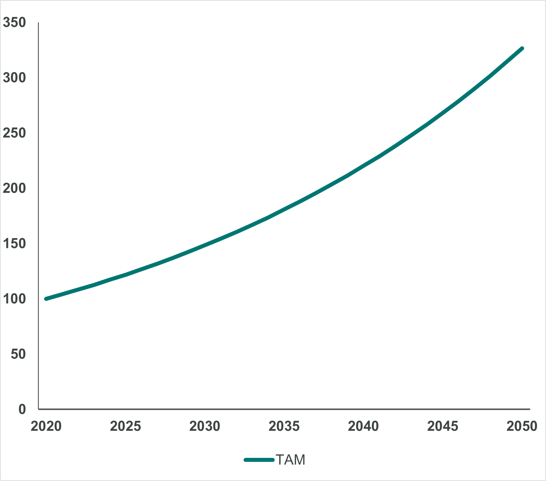
Total Addressable Market (TAM) refers to the largest possible market for a given solution. This market can be expressed as revenue, annual units sold, or the total GHG emissions generated annually by an industry or sector. As the global economy evolves and technology improves, tracking changes in the TAM and understanding their impact on GHG emissions is essential.
Serviceable Addressable Market (SAM)
SAM is the realistic portion of TAM that applies to a specific solution. To estimate the SAM, consider regulatory barriers, consumer preferences, infrastructure limitations, price, payback, and available capital or means of financing the solution. You may also consider distribution networks, production capacity, and supply constraints. Market segmentation is crucial at this step. For instance, while the TAM for new EV technology may be all road vehicles, including passenger, freight, and construction vehicles, the SAM for that solution may be passenger vehicles only. This enables a more credible and accurate unit impact analysis, e.g., using passenger vehicle weight rather than average weight across all vehicles.
Serviceable Obtainable Market (SOM)
SOM is the portion of the SAM that a specific solution can realistically serve. It is the portion of the market that the solution can realistically win, based on its value proposition, sales effort, and market readiness. In the early years of a new product, the SOM is smaller than the Serviceable Addressable Market (SAM) for several reasons, including lack of awareness among potential customers, limited distribution channels, unproven technology, and competition from established players and incumbent solutions.


2.3
The S-Curve: Market Adoption and Technology Diffusion
As the market gains awareness and comfort with new solutions and the solution overcomes barriers to adoption, the SOM and SAM may converge in time. As using a top-down measurement approach tends towards overestimating the near-term GHG impact, an analyst needs to be aware of these challenges and to focus on capturing the realistic SOM rather than assuming instant adoption into a theoretical SAM. Understanding this transition is one of the fundamentals of calculating forward-looking impact and is imperative to avoid greenwashing and greenwashing criticisms.
While there are many factors affecting a solution’s success, when and how a new proposed climate solution will be adopted by the market is probably the most significant — and the most difficult to assess. Fortunately, the adoption of new technology or the diffusion of innovation has been studied for decades, and some common approaches are routinely discussed. This theory integrates various sociological theories and behavioral change models to explain how new technological advancements spread throughout societies and cultures, from introduction to widespread adoption, through an S-curve.

This chart highlights the S-curves for various consumer products over the past century.
Theory Behind the S-Curve
The theory of the Diffusion of Technology refers to the process by which an innovation is adopted and spread throughout a market. The diffusion of innovation theory classifies adopters into five segments: innovators, early adopters, early majority, late majority, and laggards.
As shown in the figure to the right, some are likely to adopt a new technology, while others are likely to resist. The innovators are the first to adopt a new product or technology and are often willing to take risks. The early adopters are the next group to adopt, and they help to validate the product for others. The early majority adopts a new product once it is proven effective, while the late majority adopts it only after most people have already adopted it. Laggards are the last group to adopt, and they are often resistant to change.
The naturally occurring gap between the early adopters and the early majority is called the chasm. The fundamental idea of the Diffusion of Innovation theory, as it relates to investors and entrepreneurs, is that you can't change a laggard to an early adopter or even persuade the late majority toward the early majority. The product and the way a product is sold must evolve to fully advance through the cycle.
Overall adoption theory yields an S-shaped curve that represents the potential adoption of a technology — or, in this case, a proposed climate solution — over time.

Theory of Diffusion of Technology
Using a Diffusion Curve to Convert SAM to SOM
Diffusion theory provides insight into the factors that influence the rate of adoption of a new technology class or solution, such as its relative advantage over existing solutions, compatibility with existing practices, and the availability of support and information.

Hypothetical Estimate of TAM, SAM, and SOM
The diffusion curve model above is normalized to provide an adoption factor ranging from 0 to 100%. This adoption factor in each year is multiplied by the SAM in the corresponding year to develop the SOM curve, which demonstrates the diffusion of a technology into a growing market (4%/year). Depending on the parameters selected, the curves will eventually converge.
2.4
Calculating Potential Impact
Potential impact is calculated or estimated using a top-down approach: Derive the SOM for the technology class from the applicable SAM and then multiply the relevant annual volume by the Unit Impact (see Section 1) to derive the estimated potential impact (CO₂e/year).

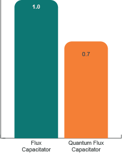
For example, consider a company that is the originator and sole producer of quantum flux capacitors, which require 70% of the energy of conventional flux capacitors. Globally, flux capacitors produce 100 T of CO₂e GHG emissions annually. The company has been around for a few years and has about 4.8% of the flux capacitor market, on an installed unit basis.
The CO₂ emissions factor for the incumbent flux capacitors informs the baseline scenario for the impact analysis. The unit emissions for production of flux capacitors and the new quantum variety are 1.0 and 0.7 tons of CO₂/unit respectively. If the one-off effect on production emissions is the only effect of quantum flux capacitors, then the unit impact for quantum flux capacitors is 0.3 tons of CO₂/unit produced, and the potential impact calculation is a straightforward multiplication of unit impact and SOM in a given year.
In order to be thorough and accurate, the analyst must model all relevant effects. If, for example, there is also a recurring effect associated with operating a quantum flux capacitor, then the impact of the solution needs to reflect a combination of both effects. Tracking impact for a recurring effect requires the analyst to build a fleet model.
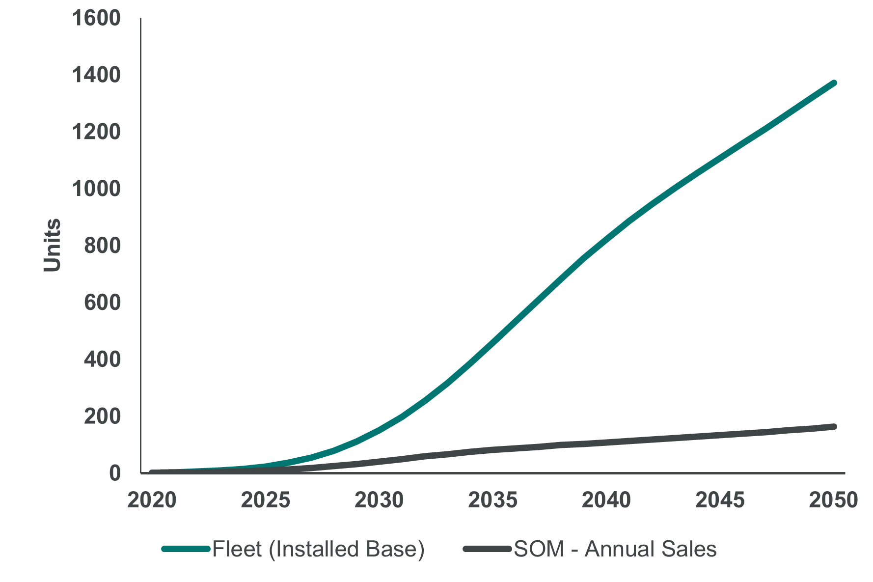
Comparing Annual Sales and Fleet Perspectives
To provide a real-world example, the primary recurring effect of solar panels is that they offset emissions from fossil fuels each year of their operating lifetime, but they also have a negative, one-time effect when they are produced. In this case, a hybrid model is needed with two components: one using annual sales for the one-time effect associated with manufacturing, and one using the size of the installed base (i.e., how many MWs of PV panels are installed) for the recurring effect associated with displacing the emissions from fossil generation.
Returning to the example of quantum flux capacitors, the model for potential impact would begin in 2020, which was the year of market entry. The S-curve is then adjusted such that this solution has 4.8% of the flux capacitor market in 2023 (present day), which increases to 100% of the market over time. By summing impact across all relevant effects, the analyst can calculate net potential impact of quantum flux capacitors in each year, e.g., 10 MT per year in 2030. As adoption or technology diffusion increases and the market grows, the potential impact of Quantum Flux Capacitors could increase to 50 tons CO₂e per year by 2050. By stating “potential impact,” “per year,” and “in 2050,” the statement is a clear and precise representation of the results of this impact calculation.

Potential GHG Impact Per Year
The underlying process typically produces a curve, but investors may focus on thresholds or goals for a certain year.
Because of the significant uncertainty in long-term market projections, Project Frame recommends constructing alternative scenarios with different market size assumptions or technology adoption rates and analyzing potential impact in each scenario. Exploration of different future market scenarios can also be paired with variation of parameters that affect unit impact. Key drivers of uncertainty will differ in each impact analysis. In some cases, the analyst may choose to vary parameters that appear in the baseline scenario, such as incumbent emissions; in other cases, they may vary parameters around a solution’s technical performance. See the sample GHG Impact Potential Analysis in the appendix for an example.
Section 3
Planned GHG Impact
Project Frame uses the term planned impact to align with the “bottom-up” method of quantifying how a unit scales, based on what the company deploying the solution intends to achieve (per a realistic analysis of its business model). Planned impact applies a bottom-up analysis of the company’s growth or business plan, assessing its current customer pipeline, expected sales, and expected growth in the coming years. This is typically well-defined in the near term, with good visibility of potential customers and sales. Planned impact aligns with SOM
market sizing based upon specific company commercial forecasts.
By aligning a company’s emissions impact with its business plan, investors can increase their confidence that impact will emerge with its commercial success. Given a predefined, per-unit emissions reduction impact, a company’s planned impact will increase proportionally with a company’s customer growth.
Vist the Project Frame website for an example of planned impact in action.

Representation of the Project Frame GHG Impact Forecasting Structure
Investors have differing targets and priorities in their selection criteria. As the calculations are based on curves, the same models can produce estimates to align with near-, mid- and long-term targets.
Deriving Planned Impact
3.1
Commercial Forecasts
Commercial forecasts are typically sourced directly from companies, and they should be assessed for feasibility, realism, past performance, and industry expectations. It is best practice for analysts to align impact modeling with financial modeling in diligence, as the logic underlying expected company growth is the same.
Here are some key questions to consider when assessing company commercial forecasts and growth:
Why was the forecast prepared? Was it prepared to operationalize or was it prepared to attract investors?
How was the forecast prepared? Is it based upon factual data or is it assuming growth rates year on year?
How does the forecast compare to historical performance? Is there historical performance to assess?
Does the forecast align with industry growth expectations?
If relevant, does the forecast account for shifting customer types over a multiyear time horizon?
Company commercial forecasts must also align with the carbon unit impact and baseline scenarios. If fundamentally different assumptions are made that underlie the carbon unit impact and the company forecast, then an investor or analyst will develop an investor-adjusted commercial forecast, which is based upon the company forecast but changed where assumptions or data are assessed to be more realistic or appropriate. Developing investor-adjusted commercial forecasts is common, and typically these adjusted forecasts are more conservative in nature.
3.2
Calculating Planned Impact
To calculate planned impact, the unit impact (from Section 1 of this paper) is multiplied by the relevant annual volumes developed from the commercial forecast to derive the impact estimate or forecast. Throughout this entire process, it is important to try to develop the simplest model that defensibly captures the proposed climate solution and baseline scenarios. Making needlessly complex models, with many immaterial or insignificant dynamic projections, may leave the model unintelligible, difficult to interpret, and difficult to update in the future.

Planned impact can then be rolled up to a total number over the measured time horizon by adding the annual planned impact.
3.3
Long-Term Planned Impact
When assessing long-term planned impact, typically defined as beyond a 5-10 year time horizon, it can be difficult to source commercial forecasts with appropriate granularity. This can necessitate combining a bottom-up and top-down analysis of a company’s forward-looking impact. This results in shifting methods to utilizing market trends, sizing, and assumed company market share — covered in the potential impact section — once detailed bottom-up forecasts are no longer available. It is common to use the company forecasts as a basis and then assume a market share like 15-30%, depending on the level of fragmentation expected in the market. Applying this market share to the SOM for the technology solution provides an equivalent SOM for the company that can bridge with the bottom-up analysis done for the first 5-10 years. This SOM can be compared to the bottom-up commercial forecast and adjusted accordingly, providing a litmus test for the company's commercial forecasts.
The figure below demonstrates what the expected result of measuring long-term planned impact would look like compared to potential impact. Potential impact for proposed solutions results in optimistic curves, while planned impact results in more conservative assessments — even when extended beyond company forecasts.
If the top-down and bottom-up planned impact analyses are combined, take caution to use the correct baseline assumptions in the unit impact calculation. It is common to use a different baseline in the unit impact calculations to estimate planned vs. potential impact. This is because of material differences in the typical unit for the technology class’s broader SOM and the target customers for the specific solution. For example, the SAM for a particular company may be specific to a region with a high CO₂ intensity of the grid, whereas the average CO₂ intensity of the grid is much lower for the broader global market. Another example is calculating the unit impact for a typical passenger car for use with the SOM of the technology class for potential impact, but using a high-performance sports car for the unit impact associated with planned impact, based on the product and market focus of a particular company.

Bridging Commercial Forecasts with Company SOM
Analysts can use the company SOM to extend the planned impact when necessary to produce extended forecasts. This approach also allows a reality check with the SOM for the broader technology class.
Section 4
Other Considerations
Attribution and Additionality
Project Frame defines attribution as, “the process of allocating credit for GHG impact based on the relative contributions of various participants in the value chain.” Attribution is also delineated into two categories; vertical and horizontal. As mentioned in our introduction, the majority of the Frame Focus Group stated that attribution is not a factor in pre-investment screening or post-investment reporting;
however, we still feel it is critical to align on best practices if and when it is used. Similarly, Additionality is only an important consideration for some investment practices, and there are many interpretations for its meaning and how it should be applied. We have reached some consensus amongst the Frame Content Working Group on this topic, which we share below.
4.1
Attribution
A solution that enables the reduction of greenhouse gas (GHG) emission rarely results from the action of a single company. A solution is often the result of the mobilization of an entire value chain, which mines, transforms, transports, feeds power, and distributes a product to a final user. A value chain is made up of several contributors in a system (see Figure 1 and 2 for illustration); each provides its added value to the product. An attribution methodology consists of a quantitative distribution rule that divides the resulting total GHG emission reduction and allocates one part to each of the solution’s contributors.
How do we distribute the GHG-avoided emission generated by a solution among all the contributors that made it possible? Naturally, each of the contributors would like to claim a part (if not the whole) of the overall GHG emission reduction. Indeed, the claim of GHG emission reduction potentially increases its attractiveness for investors or clients.
The concept of attribution was one of two areas shared with the Frame Focus Group. When asked if the investors considered attribution as a factor pre-investment, 47% of respondents said yes, whereas 40% said that attribution was a factor in post-investment reporting. Will this percentage shift with the increase of regulation and competitive carbon markets? We intend to dive into motivations further as part of our Frame annual survey in 2023.
Horizontal attribution
Attributing portions of emissions reduction impact across contributors along the value chain.
Vertical attribution
Attributing portions of impact across the shareholders of the company that has put the proposed climate solution on the market.

Illustration of Vertical and Horizontal Attribution of GHG Emissions Reduction
When deciding whether or not to claim GHG impact attribution to an investment, we should first ask: Why is this important? Why can’t all the contributors along a value chain claim the final result in its entirety? How can we claim attribution with rigor and transparency?
First, each contributor, large or small, decisive or accessory, can claim the same effect, independent of the nature of their contribution — a circumstance known as multiple counting. For example, the actual GHG emissions reduction generated by the installation of one new windmill could be claimed in parallel and cumulatively by (1) the windmill manufacturer, (2) the investor that financed the wind park, (3) the operator that built it, and potentially (4) the steel producer that provided the steel for the mast.
An outside reviewer of these claims may assume that they can add the value of each contributor, causing an overestimated (overoptimistic) picture of our ability to reach a Net Zero objective. Hence, partitioning the final effect among the various contributors would help render a true picture of impact.
Second, investors who consider the climate effect during the arbitrage of their financial return will implicitly give a value to the GHG emissions reduction they enable through their investment. The reduction of one ton of GHG emissions will then have a monetary value. As a consequence, our accounting for the GHG emission reduction shall be at least as quantitatively robust as our accounting for the money.
Finally, as we aim to ensure our Net Zero objective, we should efficiently allocate capital through all the contributors in terms of GHG emissions reduction. In order for this flow of capital to reach the right contributors according to the importance of their contribution, we should build a methodology for distributing a given solution’s total GHG emission reduction among all of its contributors and ensuring that the sum of these contributions will equal the total GHG emissions reduction. In other words, in addition to being non-cumulative, the distribution also shall be meaningful and produce the impact we seek.

Illustration of a Generic Chain of Contributors

Illustration of an Example Chain of Contributors in the Heat Pump Sector
4.1.1 Horizontal Attribution
There are various attribution methodologies for allocating GHG emission reduction along a value chain.
A good attribution methodology shall:
Avoid multiple counting (“perfect partitioning”) so that each ton of GHG avoided is allocated only once and that the sum of all claims is equal to the resulting GHG emission reductions.
Reward the most impactful contributors, meaning that the capital shall go preferentially to the contributors that produce an amplifying effect, such as removing a bottleneck in a value chain or substantially improving performance.
Be practical. Use readily available data and limit the margin for interpretation.
Among today’s various proposed methodologies, there are several possible options, described below. As no single method has been recognized industry-wide, the end user must choose its own method and report transparently on it.
No horizontal attribution: Give up, as it’s too complex.
Stakeholder consensus: Establish a distribution key that all horizontal contributors agree upon in a collective approach. (For example see: World Resources Institute’s “Estimating and Reporting the Comparative Emissions Impacts of Products” and Mission Innovation’s “The Avoided Emissions Framework.”)
Equal allocation: Use an equal split of the total GHG emissions reduction among the main group of horizontal contributors. For example: raw material (33%), manufacturer (33%), and distributor (33%).
Targeted allocation: Allocate all avoided emissions to fundamental solutions or use of a predefined rule. (See Schroders/GIC, A Framework for Avoided Emissions Analysis)
Cost prorate: Distribute the total GHG emission reduction using the prorate of the cost of each contributor to the total cost of the solution.
Currently, there is no existing method that satisfies the criteria above indisputably.
The criterion most difficult to fulfill is the preferential routing of capital through the most impactful contributor in order to achieve the most emissions reduction. That’s because the criteria is highly subjective. Although the measure of impact is hard to quantify, some criteria can help qualify it. For example, a pioneer originating a new low-carbon solution should be qualified as an impactful contributor. In the same spirit, a company that has developed, over the years, a unique know-how without which the solution couldn’t be implemented should also qualify as an impactful contributor. These impactful contributors should be rewarded.
Given the complexity of a horizontal attribution methodology, Project Frame does not recommend at this time horizontal attribution based on a quantifiable approach. We instead recommend that the role of the solution in the chain of contributors is described in relatable, transparent terms. It is also important to acknowledge the role of proposed climate solutions other than the one being scrutinized, to achieve the resulting GHG emissions reduction.
4.1.2 Vertical Attribution
Attribution among the equity owners of a company
Shareholders may need to report and aggregate the GHG emissions reduction of its portfolio companies together. How do we share the GHG emissions reduction achieved by a given company among its shareholders?
As depicted in the image below, the simplest solution appears quite easily: distribute credit for emissions impact according to the investor’s ownership.
However, there are some limitations to this method, including the following:
Some investors (e.g., seed, VC) have taken on higher risk earlier and made possible the rapid emergence of a given solution. Some could argue that this early positioning should receive more credit.
The financing of a given company is not only done through equity but also through other forms of investments that do not result in ownership, such as grants, tax credits, or debt. One could argue that the taxpayer should be rewarded as well for their contribution through public funding. The concepts of concessional or catalytic capital, referred to by the Emerging Climate Technology Framework, Prime Coalition, and others, can be used to manage this challenge.
An investor through its investment at year (y) makes possible the emergence of an impact that will last over the years (y+n). The same investor may sell its share after a while, and the question then could be whether the produced effect of its early financing should continue over time as a kind of carbon patent. This could be a way to support early investors that are willing to take a high level of risk.

Illustration of Attribution Among Shareholders
Note: Project Frame endeavors to provide recommendations for how investors should report and aggregate the realized GHG emissions reduction of their climate solutions and portfolio companies. This reporting of GHG emissions reduction does not constitute a form of offset asset that could be used to decrease other GHG emissions reduction. Frame discourages this practice because it is currently impossible to supply this data in a reliable and auditable way; without a clear and reliable process, this trend can lead to further “greenwashing” or “impact washing,” derailing progress made by diligent actors in the climate investing space. This practice also could deter investors from allocating capital to critical solutions that might aid in emissions reduction even if they do not cause the reduction directly.
Frame does not intend to promote the practice of attributing GHG impact to a dollar value or particular investment. As stated in this paper's opening, the majority of investors currently do not consider attribution when screening proposed climate solutions pre-investment. Frame's minimum recommendation is for investors to report the aggregate of their portfolio companies' potential and/or planned GHG impact and the portfolio companies' realized or actual GHG emissions impact during the year when the effect has been produced. Reporting further details on the total impact by subcategories, such as GHG impact type, solution type, geography, etc., are highly encouraged. It should be made clear they are reporting the total impact of their portfolio companies without attributing the impact uniquely to their investment.
Based on the feedback received from the Frame Focus Group, investors wishing to claim attribution can report a percentage of their portfolio companies' achievements using their equity ownership proportion in these companies during the year when the effect has been produced. This can be complemented by qualitative inputs detailing the additional contributions of the investor to ensure the proposed climate solution's or company's success. This continues to be an area of strong debate among the Frame community, and we will continue to update guidance in the future.
4.2
Additionality
In this section, our intention is to provide context, considerations, as well as questions to facilitate thoughtful examination of the term and its application. We will also provide some recommendations to minimize “greenwashing” or the appearance of such.
A proposed climate solution or other climate intervention is said to be additional if the GHG reduction would not occur but for the deployment/existence of the proposed climate solution or intervention. If the reductions would happen anyway, then the proposed climate solution’s GHG reduction is not additional.
However, additionality has different uses in different climate contexts, including:
In reference to carbon credits and/or carbon offsets: Usually, the organizations that certify carbon credits or offsets have specific rules about what qualifies as “additional.” This chapter does not address this use of additionality. For more information on additionality requirements for carbon credits or offsets, refer to the certifying organization.
In reference to the impact an investment fund has on GHG emissions: This is closely related to attribution of an investment fund’s impact, which is covered earlier in this document. This section does not address investment fund additionality, which is closely dependent on the additionality of the proposed climate solutions in which the fund invests. In this context, additionality often gets conflated with providing added value. Rather than using the term additionality to articulate your firm’s enhancing contribution to an investment or company, it is recommended to use the term “added value” or “value add.” These terms more accurately describe the contributions being made, for example, in terms of knowledge sharing or network-building.
In reference to the impact of a proposed climate solution: Organizations propose climate solutions and seek funding to support the development and deployment of the solutions. Potential investors should assess the additionality of a proposed climate solution to determine the GHG reductions that occur based on the existence of the proposed climate solution. This section addresses the issues to consider when evaluating additionality of proposed climate solutions.
The concept of additionality is closely tied to the evaluation of potential or planned GHG impact (Section 2), and, in fact, there is usually significant overlap between the analyses. However, when determining potential or planned GHG impact, a baseline is used that may not be broad enough to account for all potential GHG flows or other possibly unconsidered factors that could significantly affect GHG impact. An additionality analysis is an extra lens to view the proposed climate solution, to ensure the consideration of key factors that affect the net benefit of the solution.
4.2.1 Determining Additionality
While simple in concept, determining additionality can be complex in practice. How can we be sure that a solution is offering something for the future that other solutions are not — especially in a world where GHG reductions are occurring all the time? New laws and regulations will impact emissions, as will changing market conditions and the availability of alternative solutions.
The process of determining additionality can be subjective and will depend heavily on assumptions such as the baseline case (or cases) of comparing incumbent solution(s) with the proposed climate solution. Assumptions will also need to be made about future market conditions, alternative solutions, grid conditions, government regulations, and other factors.
The following issues should be considered when assessing the additionality of a proposed climate solution:
Out of all the concepts presented in this iteration of the methodology, the concept of “additionality” is the most debated; we have not yet reached consensus on a final definition, or on ways to consistently or systematically assess additionality. We look forward to continuing this discussion with the community.
Laws and Regulations
Governments may require GHG reductions in various markets, so introducing a proposed climate solution in that market may not result in additional GHG reductions. For example, some governments are banning the sale of ICE vehicles starting in 2035. Therefore, a company offering battery electric vehicles (BEVs) as a lower-emission alternative to ICE cars may not be able to consider GHG emissions reductions after 2035 to be additional in affected territories.
Alternative Solutions
If the alternative to using the proposed climate solution is to use another solution with similarly low GHG emissions, then the proposed climate solution may not be additional. For example, if a customer would buy an alternative BEV from another company if the proposed climate solution company’s BEV was not offered for sale, then the GHG reductions from the sale of that company’s BEV are not additional. However, if the supply of low GHG-emission alternative solutions is limited, then a proposed climate solution that increases supply (even in the presence of low-emission alternatives) would be additional.
Creating New Energy Demand (Rebound Effect)
A proposed climate solution that offers reduced GHG emissions compared to an incumbent may sometimes encourage people to switch from other low or zero GHG options to a higher emissions product. To the extent a proposed climate solution takes market share away from solutions that emit even less, it does not lead to better outcomes, and that portion of its market is not additional.
For example, in 2021, the No.1-selling BEV in China, the Wuling Hongguang Mini EV (see photo to the right), cost approximately $5,000. While that low price likely made many prospective ICE car purchasers choose the low-cost BEV instead, it may have also encouraged bicycle or e-bike riders to stop riding and buy a BEV instead.
Elimination of Barriers to Market Entry
Barriers to entry for climate solutions are falling as costs drop and regulations for fossil fuel energy increase. In the past, when renewable (wind and solar) energy was significantly more expensive than fossil fuel-based electricity, organizations deploying renewable energy would count such systems as additional. Today, wind and solar electricity is often significantly less expensive than coal and natural gas-based electricity. Depending on where the technology or service is deployed, new deployments of renewable energy may not be additional. Of course, renewable energy still has significant environmental advantages over fossil fuel-based energy, so it still should be encouraged.
While lower GHG solutions may be commercially available and less expensive than incumbent solutions, they still may not be implemented under a business-as-usual scenario (i.e., without the proposed climate solution) due to other barriers such as information costs/limitations, financial constraints, social acceptability, or regulatory restrictions. In those cases, GHG reductions from a proposed climate solution that address those other barriers may be considered additional.
Note that being first to market is not the determining factor in additionality. BEVs were popular in the early 1900s (see photo below). A century later, the relatively affordable Nissan Leaf went on sale in 2010 before the expensive Tesla Model S was introduced in 2012, yet Tesla’s entrance into the automobile market created a large impact that has and will significantly lower emissions in the transportation sector.

The $5,000 Wuling Hongguang Mini EV

Battery Electric Vehicle Advertisement from McClure’s Magazine 1912
4.2.2 Other Additionality Examples
Carbon Capture
Additionality of carbon capture systems — such as point-source Carbon Capture and Sequestration (CCS) or Direct Air Capture (DAC) — are usually easy to assess. Such carbon capture systems directly remove CO₂ from the air (DAC) or prevent CO₂ from entering the atmosphere (CCS). Such systems are often considered additional since the emissions would occur or remain but for the existence of the carbon capture system. If the existence of the carbon capture system ultimately is used to justify further use of fossil fuels when lower GHG alternatives are available, however, then the additionality may be questioned.
A DAC system, when used to remove past emissions from the atmosphere, is almost certainly additional, as the amount of past emissions is huge (approximately 2.4 trillion tons of CO₂). Therefore, any amount of DAC (taking into account any emissions from the DAC system) will provide a beneficial reduction of atmospheric CO₂.
Video Conference Software
The use of video conference software (VCS) can replace traveling to a meeting or conference and, therefore, could result in significant emissions reduction. While it is relatively easy to calculate the emissions savings from using VCS compared to flying to a business meeting, determining the additionality of VCS emissions reduction is more nuanced. Some of the factors to consider:
What percentage of meetings would not otherwise occur if VCS was not available?
If you are assessing a new VCS product meant to compete with Zoom, FaceTime, or other existing products, how much will the new product reduce travel on top of the impact of the current products?
To the extent that new laws, regulations, or rules are implemented to require use of VCS instead of travel, those reductions should not be considered additional.
VCS can have a rebound effect. To the extent that VCS allows people to do business with people or organizations outside their local area, those wider-area relationships may result in additional travel to meet the people or organizations, even though the majority of the interactions are by VCS. In this case, the VCS allowed interactions to take place that would have not otherwise taken place, so the VCS calls are not additional; furthermore, the resulting travel should be considered to be increased emissions due to the use of VCS.
Frame recommends providing a definition for how your firm interprets and applies additionality before making any claims. Firms should also reevaluate and capture their decision-making process regularly. Developing a consistent framework or using a decision-making tool can assist the process.
Appendix
Unit Impact
Examples of Generated Effects for Impact Scope
Ultra Low-Leak Valves
A valve for gas distribution pipelines that provides an extremely good seal over the current, business-as-usual valve.
|
Description |
Reduce/ Increase |
Recurrence of Effect |
How is it quantified? |
|
|---|---|---|---|---|
|
Effect A |
The leak rate of the pipeline will be lower due to the better seal provided by the new valve |
Reduce |
Recurring The effect will be produced over the whole lifetime of the valve |
Estimated – GHG impact can be estimated based on average performance of the company’s valve in similar market conditions to the traditional valve |
|
Effect B |
The production of the valve uses 10 kg more steel than the business-as-usual valve |
Increase |
One-off This effect only occurs once, at manufacturing stage |
Estimated – GHG impact can be estimated based on average carbon intensity of steel per kg |
|
Effect C |
A heavier valve will mean that more fuel is used in transportation |
Increase |
One-off This effect only occurs once, during transportation |
Not Quantified Unlikely to make a material difference |
Low Carbon Cement
A hypothetical low carbon cement that has a carbon footprint 50% lower than regular Portland cement, with the same durability and strength qualities.
|
Description |
Reduce/ Increase |
Recurrence of Effect |
How is it quantified ? |
|
|---|---|---|---|---|
|
Effect A |
The cement has half the carbon footprint of regular Portland cement which it is displacing (the unit is per tonnes of cement) |
Reduce |
One-off This effect only occurs once, at manufacturing stage |
Estimated – GHG impact can be estimated based on average performance of their cement in similar market conditions to standard Portland cement |
|
Effect B |
This process requires 2% less water than regular Portland Cement |
Reduce |
One-off This effect only occurs once, at manufacturing stage |
Not quantified Unlikely to make a material impact |
Industrial Production Energy Efficiency Software
A software program used to optimize industrial production processes in order to reduce carbon.
|
Description |
Reduce/ Increase |
Recurrence of Effect |
How is it quantified? |
|
|---|---|---|---|---|
|
Effect A |
The software can reduce manufacturing inputs by 5%, reducing over design |
Reduce |
One-off This effect only occurs once, at manufacturing stage |
Directly Measurable – GHG impact can be directly quantified by the software |
|
Effect B |
The software can reduce manufacturing process times by 2%, reducing the amount of energy used |
Reduce |
One-off This effect only occurs once, at manufacturing stage |
Directly Measurable – GHG impact can be directly quantified by the software |
|
Effect C |
The software itself uses energy to run |
Increase |
Recurring |
Not Quantified Unlikely to make a material difference |
Industrial Production Energy Efficiency Software
A software program used to optimize industrial production processes in order to reduce carbon.
|
Description |
Reduce/ Increase |
Recurrence of Effect |
How is it quantified? |
|
|---|---|---|---|---|
|
Effect A |
The software can reduce number of damage events for gas distribution (such as repair workers digging into pipes by accident) |
Reduce |
One-off |
Estimated – GHG impact can be estimated based on average leak rate per event multiplied by the number of events that have been avoided |
|
Effect B |
The software can reduce the need for repair crews to go out and fix damaged pipes |
Reduce |
One-off |
Not Quantified Unlikely to make a material difference |
|
Effect C |
The software itself uses energy to run |
Increase |
Recurring |
Not Quantified Unlikely to make a material difference |
Life Cycle Analysis (LCA) and Emissions Factors
How are Emissions Factor Data Obtained From LCAs?
The US National Renewable Energy Laboratory defines a life cycle assessment (LCA) as a “systematic gate-to-gate, cradle-to-gate, and cradle-to-grave process that evaluates the environmental impacts of products, processes, and services.” In short, it is a methodology that allows one to track the environmental impact of a product over the course of its entire life cycle, starting from resource extraction to create the product and going through to the product’s disposal. It quantifies both the energy the life cycle uses and the pollution that it yields. Overall, it is a powerful tool used by many in government, industry, academia, and advocacy to reduce resource consumption and pollution.
Unlike the forward-looking impact methods being developed by Project Frame, life cycle analysis/assessment is a well-established field with well-defined practices. An LCA must fulfill the standards laid out in ISO 14040 and 14044. The LCA field also has a broader scope than Project Frame’s focus on GHG emissions, as LCAs can calculate emissions of all types (GHGs, smog, particulate matter, etc.) as well as resource use.
LCAs consist of four primary components:
Goal and Scope Definition: LCAs must first outline their purpose, which could be broad (e.g., total emissions of a production process, including all water, land, and air pollutants) or narrow (e.g., CO₂ emissions change from electrifying a single process step). LCAs may be designed in order to assess the total emissions of a product, the emissions of a particular step in its production, or the relative emissions of several different production methods. The system boundary of the LCA depends on its goal.
Inventory Analysis: The emissions of the inputs of the system are gathered through direct data collection, or, more commonly, modeling with LCA software.
Impact Assessment: The emissions in the inventory list are normalized to the unit of analysis and compiled into a set of final values. The LCA practitioner has significant leeway here and can choose exactly how they want to report these values.
Interpretation: Final results are interpreted and discussed for the benefit of the reader. Discussion of the uncertainty bounds of the analysis and any particular difficulties can be especially helpful in order to place the values in context.
LCAs may prove useful in a variety of ways when constructing a forward looking analysis. Consider the following climate solutions and the possible applications of LCA data:
Proposed climate solution: Carbon fiber plastic composites that enable a lighter-weight chassis on battery electric vehicles.
An LCA of carbon fiber composites could provide an emissions factor for the composites.
LCA of battery electric vehicles (BEVs) may be able to inform what proportion of emissions in BEV manufacturing come from the chassis.
If the LCA is cradle-to-gate (see below), it could also give information about average operational mileage and driving emissions.
Projections of grid emissions factors may be necessary to calculate BEV charging/operational emissions.
Proposed climate solution: Membrane technologies reduce the energy input necessary for industrial chemical processes.
One could look at LCAs for specific chemical products to identify energy usage in the affected processes.
If top-level fuel savings are known, emissions factors would be used to convert fuel usage — in units of quantity used (kg, MT, etc.) or heat produced (kWh, MMBTU, etc.) — to CO₂e emissions.
Proposed climate solution: Efficient power conversion for data centers.
LCAs may provide rates of energy consumption per data center, server rack, or server. Other industry or academic research (not LCAs) may also prove invaluable to estimating total industry energy usage.
Projections of grid emissions factors may be necessary to calculate operational emissions in the future.
LCA Resources
Emissions factors can be found in a number of sources, including:
Government Agencies: Many national and regional governments have published emissions factors for various activities and processes in their jurisdiction. For example, the US Environmental Protection Agency (EPA) provides a database of emissions factors for various sources.
International Organizations: International organizations, such as the United Nations Framework Convention on Climate Change (UNFCCC), also provide emissions factors for different sectors and countries.
Research Institutions: Research institutions and universities often conduct studies on emissions factors and may have their own databases or reports.
Industry Associations: Industry associations, such as the Electric Power Research Institute (EPRI) or the International Energy Agency (IEA), often provide sector-specific emissions factors and related information.
Commercial Providers: Some commercial providers also offer databases and tools to estimate emissions factors and assess the environmental impact of specific activities.
Standards and Guides
There exist many principles and frameworks for conducting a thorough LCA. This section lists a variety of documents (some free) that can help guide the process. One highly relevant guide is “Life Cycle Assessment: Principles and Practice,” written by the Scientific Applications International Corporation (SAIC) for the National Risk Management Research Laboratory (NRMRL) of the US Environmental Protection Agency (EPA). Not only does it cover the relevant definitions and processes, it also provides links to software and additional references for those that wish to learn even more.
As noted, the leading standards for LCA come from the International Standards Organization (ISO), and are ISO 14040 and ISO 14044, which cover the principles and framework for LCA (14040) and the specific requirements and guidelines for LCA (14044). Official versions of these documents are available for purchase from ISO.
There are also many product-specific or country specific standards. PRé Sustainability has an article that summarizes and acts as a jumping point for many of these standards.
Software and Tools
Appendix B in the SAIC 2006 has a table of tools for conducting an LCA. LCA software can greatly expedite the process of conducting an LCA, as the frameworks, calculations, and data are easier to access and integrate; however, the learning curve for using LCA software is steep. Outside of the software listed by the EPA guide, there exist many websites that list a few tools along with how to access them.
SimaPro (by PRé) and GaBi (by Sphera) are industry standard LCA tools. Another tool worth noting is openLCA, which is free and open source. Most of these tools refer to databases that catalog product emissions. OpenLCA also lists example databases that are used, including both free and for-purchase databases.
Additional Resources
Outside of using these tools and standards, there are many papers and studies that document parts of or entire LCA processes. Journals include The International Journal of Life Cycle Assessment, and the Journal of Cleaner Production. Searching for LCA results through Google Scholar also brings up many studies that address the LCA of specific products.
For more information, here are several resources and tools for finding emissions factors and life cycle analyses:
Idemat (mobile only)
Journal of Industrial Ecology
Journal of Cleaner Production
Journal of Environmental Science & Technology
Converting Units with Dimensional Analysis
This section provides a brief overview of how dimensional analysis can be applied to better leverage and enhance accessible data sets, with the intention of estimating the planned or potential GHG impact of climate solutions.
Dimensional analysis is a basic problem-solving approach that relies on known mathematical relationships between two units that describe equivalent “amounts” in the numerator and denominator, each with a different unit of measure. These relationships are known as unit factors. Dimensional analysis can be a powerful tool for linking disparate pieces of information in such a way thatresults in a credible (if not perfectly accurate) set of metrics. Familiar examples are volumetric conversions in baking, stoichiometry in chemistry, and simple unit conversions between metric and US standard.
When converting between units, the analyst should be cautious. Forward-looking GHG impact calculations can require a vast array of parameters and contain many variables, often relying on information from several disciplines. Unit factors for forward-looking impact assessment can be divided into a few major categories: exact and approximate constants (e.g., inches to feet, US pounds to kilograms), material- or process-specific properties (e.g., density, energy content), and life cycle factors (e.g. gCO₂e/kWh).
One simple example is identifying the emissions per unit of electricity from a natural gas combined-cycle power plant. The power plant has a heat rate of 7580 BTU/kWh. Natural gas has an emissions factor of 52.91 kg CO₂e/MMBTU. Dimensional analysis allows the analyst to obtain the emissions factor in terms of T CO₂e/MWh:

Here are a few best practices to help ensure that, later on, others are able to follow the chain of logic:
Always include units when providing numerical values; these should be shown as precisely and clearly as is feasible and follow existing conventions.
Ensure that all units cancel in the intended way; if the conversions are displayed in a linear fashion, it can be helpful to show the cancellation of units with strikethrough formatting (i.e., strikethrough).
Provide a list of acronyms, abbreviations, and units of measure in models.
Cite the source of the information.
Use simple models that are based on critical thinking and that provide clear documentation. These provide a great foundation for more complex models later on (and are sometimes more than sufficient for the task).
Do not confuse common terms that have different meanings based on geography or context. For example, a “ton” may refer to any of the following: 2,000 pounds (908.18 kg) in the US, 2,240 pounds (1,016.05 kg) in Britain, or 1,000 kg in most other countries; the latter (“metric ton”) is Project Frame’s default for measuring GHG quantities. Likewise, 1 US gallon is equivalent to 0.832674 imperial gallons.
Take care when assuming the meaning of a particular prefix within a unit of measure. For example “M” can mean “Mega” (as in million), “thousand” as in MCF for thousand cubic feet (M is the Roman numeral for 1,000), or even “metric” as in MT for metric ton.
Resources for Setting Dynamic Baselines
In some instances, a dynamic baseline for an incumbent technology is desirable over a static baseline. In reality, unit impact can change from one year to the next, simply because the product or service being displaced or improved is expected to become less GHG intensive, even in the absence of the solution. For more information on when it may be valuable and advisable to use a dynamic baseline or dynamic baseline scenario, please see Section 1.5.1 Dynamic vs. Static Variables.
There are a number of resources available either for purchase or for free, which provide reputable historical data and/or projections for both market demand and corresponding industry emissions, including for various scenarios:
Potential Impact
Calculating an S-Curve
Diffusion theory provides insight into the factors that influence the rate of adoption of a proposed climate solution, compatibility with existing practices, and the availability of support and information. Understanding these factors can help a company determine the potential rate of adoption for solutions and estimate its SOM from its SAM.
In a top-down market analysis, determining the inflection points of an S-curve is a critical input to the model. Three parameters determine the “shape” of the S-curve:
Saturation: This represents the highest market share that the innovation is expected to achieve after the product becomes mainstream.
Hypergrowth: This parameter roughly represents the beginning of the growth stage (in years) and corresponds with ~10% of expected final market penetration, in most cases.
Takeover Time: This parameter roughly represents the midpoint of the growth stage (in years) and corresponds with ~50% of expected final market penetration, in most cases.

Technology Diffusion
Illustration of a simple model used to express an S-Curve.
Adoption = Saturation/(1+81^((Hypergrowth+Takeover/2-Year)/Takeover))
Year = The number of years into the process to be evaluated
Determining the correct rate of diffusion in a scenario depends on several factors, including the nature of the solution, its target market, and the competitive landscape. An analyst would consider the level of customer awareness and understanding of the solution across different market segments/geographies, the degree of innovation it represents, its relative advantage over existing solutions, its compatibility with existing systems and processes, and its relative complexity. The analyst would also consider the marketing and distribution efforts of the company, as well as any regulatory or legal barriers that may affect its adoption.
Investors and analysts must consider several factors when formulating the adoption rate. These factors can frame the discussion:
Relative Advantage: The degree to which the new solution is perceived as superior to existing solutions.
Compatibility: The degree to which the new solution fits with existing values, experiences, and needs of the target market.
Complexity: The level of ease or difficulty in using and understanding the new solution.
Trialability: The extent to which the solution can be tested before adoption.
Observability: The extent to which the results of using the new solution are visible to others.
Marketing and Promotion: The effectiveness of the marketing and promotional efforts by the company.
Support: The availability of technical support and other resources needed to adopt and use the new solution.
Competition: The presence of competitors in the market and their impact on the adoption of the new solution.
Economic Incentives: The financial and economic benefits of adopting the new solution.
Regulation: The impact of government regulations and policies on the adoption and diffusion of new solutions.
For example, analysis of the commercial HVAC market (TAM) might be segmented into subsectors (SAM) (e.g., offices, retail, hotels and hospitality, schools and universities), with different assumptions of the adoption rates for each subsector (e.g., universities may be earlier adopters, with better funding, centralized campuses, and stronger climate commitments; elementary schools may be slower adopters with limited budgets and high market fragmentation with smaller sites). An evaluation of solutions for steel decarbonization might consider the existing use of blast furnace vs. electric arc furnace, its relative prevalence across geographies, and the decarbonization impact, given current carbon intensity for each solution.
In a top-down market analysis, determining the inflection points of an S-curve is a critical input to the model. The three parameters of saturation, hypergrowth, and takeover time determine the “shape” of the S-curve — and therefore the rate of growth and number of new and existing customers, which compounds the cumulative avoided emissions over a given time.
Rather than tweak the parameters for each innovation, analysts may find it simpler to develop a few default scenarios to evaluate, such as standard, slow, and accelerated models. These parameters were used in the chart above:
| Tech Diffusion |
Saturation |
Hypergrowth |
Takeover |
|---|---|---|---|
|
Slower |
100% |
6.0 |
12.0 |
|
Standard |
100% |
5.0 |
11.0 |
|
Accelerated |
100% |
4.2 |
9.4 |
Sample GHG Impact Potential
Produced by Prime Coalition

Inquiry
What is the magnitude of potential emissions reduction or carbon removal that could result from deployment of this solution at scale?
Solution: Capture carbon from indoor air systems
Serviceable Market: Commercial Buildings
Unit of Deployment: Individual carbon capture/air purification units
Incumbent Displaced: N/A
Analysis Date: May 2022
Full Model: Available as a Python notebook via Google Colaboratory
Prime Coalition’s approach to measuring GHG impact potential is aligned with the principles and values of Project Frame. To assess GHG impact potential, we establish a plausible baseline scenario (i.e., what market conditions might exist in the absence of this solution) and then compare this baseline scenario to a plausible impact scenario (i.e., what market conditions might be enabled by deployment of this solution at scale). The difference between the baseline scenario and the impact scenario is the potential GHG impact of the solution.
Summary of Findings
We conclude that carbon capture from indoor air circulation has gigaton-scale GHG impact potential.

Annual GHG Impact Potential

Cumulative GHG Impact Potential
The solution has two distinct impact pathways:
Each individual unit directly captures CO₂ from the circulated air inside buildings;
The integration of these units will reduce the energy needs of the existing HVAC system because the circulated air has already been heated or cooled.
Depending on the assumptions made, impact can be primarily driven by either of these two mechanisms. If the grid is extremely clean (modeled in the low-impact scenario), HVAC energy usage is not a significant source of emissions, and emissions reduction primarily comes from carbon capture. However, if grid intensity is high, the resultant energy savings can contribute to very large emissions reductions.
Assumptions
We make the following assumptions for our model:
Deployment begins in 2025.
A single unit will be able to absorb 15 MT of CO₂ per year and will require transport of 40 MT of input and waste materials over a distance of 250 miles.
Integration of technology will boost HVAC system efficiency by 25% (low-impact and baseline cases) or 50% (high-impact cases).
This technology is not well-suited for certain climates. This model limits its applicability to 70% of total commercial floor area.
Global commercial floor area is 194 billion square feet (twice that of current US commercial floor space).
Each unit services 20,000 square feet and consumes 1,500 kWh/year.
Energy use of commercial building HVAC remains constant at 0.055 quads per billion square feet.
The portion of HVAC energy consumption from natural gas remains constant at 30%.
To establish the maximum possible impact of this solution, we assume eventual full-scale deployment, i.e., 100% capture of the market for commercial buildings in relevant climates. In the absence of foresight about the specific pace of adoption for this solution, we model deployment using an S-curve with default parameters: 0.5 steepness and 50% of maximum market penetration by 15 years after initial deployment.

Scenarios
We vary the following parameters in exploring GHG impact potential, as we believe these to be key drivers of impact as well as key areas of uncertainty:
Grid intensity: We model future grid emissions using the IEA’s Stated Policies and Sustainable Development scenarios (dirty and clean grids, respectively).
HVAC energy savings: There is some uncertainty about the magnitude of HVAC energy savings expected when this technology is installed into buildings.
| Parameter | Low-Impact Scenrario | Medium-Impact Scenario | High-Impact Scenario |
|---|---|---|---|
| Grid emissions factor by 2050 (MMT CO2e/TWh) | 0.02 (IEA Sustainable Development) | 0.23 (IEA Stated Policies) | 0.23 (IEA Stated Policies) |
| HVAC Energy Savings | 25% | 25% | 50% |
| Potential GHG Impact (cumulative MMT CO2e in 2050) | 1,437 | 2,271 | 3,615 |
Acknowledgments
Project Frame would like to thank the following individuals and organizations for their expert contributions to this iteration of our shared methodology.
Authors
Keri Browder
Prime Coalition
Rick Cutright
Climate Investments (CI)
Jean-Baptiste Curien
Nysnø Climate Investments
Anna Goldstein
Prime Coalition
Dan Miller
The Roda Group
Seth Sheldon
Rho Impact
Morgan Sheil
Energy Impact Partners
Michael Solomenstev
Prime Coalition
Contributors & Internal Reviewers
Justine Davids
Carbon Direct Capital
Yi Jean Chow
Clean Energy Ventures
Anjali Deshmmukh
Prime Coalition
Shanbor Gupta
Clean Energy Ventures
Alexandra Harbour
Prelude Ventures
Matthew Harwood
Climate Investments (CI)
Lene Hodge
Nysnø Climate Investments
David Miller
Clean Energy Ventures
Adam Palay
Breakthrough Energy Ventures
Richard Searle
Climate Investments (CI)
Outside Reviewers
Melina Sánchez Montañés
AENU
Nicole Systrom
Galvanize Climate Solutions
Daniel Valenzuela
World Fund
Neil Yeoh
OnePointFive
Focus Group
Some organizations had multiple people participate
2150, AENU, Astanor, Autodesk Foundation, Azolla Ventures, Bridges Fund Management, Clean Energy Ventures, Climate Technology Group and Grantham Research Institute, Energy Impact Partners, Future Energy Ventures, Just Climate, London School of Economic, MUUS Climate Partners, Nysnø Climate Investments, OGCI Climate Investments, OnePointFive, Prelude Ventures, Prime Coalition, Starshot Capital, Thomas Goetz, VertueLab, Vidia Equity, World Fund.
Additional thanks go to the Project Frame Steering Committee, especially Sarah Kearney and Matthew Harwood for their supportive leadership and Siri Kalvig and Peter Foxpenner for authoring our Foreword, the Prime Coalition team working behind the scenes to make this paper a reality, Anjali Deshmukh, Kelsey Litwin, and Sultan White, Studio Tomo for copy editing and Genaesis Creative for graphic design. Last, but certainly not least, we want to thank our Project Frame community for their interest, encouragement, and commitment to investing for our climate.
If you are interested in getting more involved with Frame’s work, please visit Project Frame’s website to stay up to date on our upcoming content, opportunities, and events.
Project Frame is a nonprofit program convened by Prime Coalition, a nonprofit 501(c)(3), catalytic investor, and co-creator of the CRANE tool.
Project Frame does not accept direct funding from its members. Rather, it operates through grants provided to Prime. We thank those who wish to make a donation to support Prime Coalition’s work and join our shared mission to advance impact accountability in climate investing. Donations by Frame community members will be anonymized to program staff. Additional inquiries can be sent to impact@primecoalition.org.
Thank you again for your support and your commitment to investing for our climate.
Acronym Key
A - E
APS: Announced Pledges
AR6: Sixth Assessment Report of the Intergovernmental Panel on Climate Change
BEV: Battery Electric Vehicle
BTU: British Thermal Unit
CCS: Carbon Capture and Sequestration
CDM: United Nations Clean Development Mechanism
UN: United Nations
CDP: Carbon Disclosure Project
CH₄: Methane
CO₂: Carbon Dioxide
DAC: Direct Air Capture
EPA: United States Environmental Protection Agency
EPRI: Electric Power Research Institute
SAIC: Scientific Applications International Corporation
ETP: Energy Technology Perspectives
EV: Electric Vehicle
G - M
GHG: Greenhouse Gas(es)
GTI: Gas Technology Institute
GWP: Global Warming Potential
HVAC: Heating, Ventilation and Air Conditioning
ICE: Internal Combustion Engine
IEA: International Energy Agency
IIASA: International Institute for Applied Systems Analysis
IPCC: Intergovernmental Panel on Climate Change
IPO: Initial Public Offering
ISO: International Standards Organization
kg: Kilogram
kWh: Kilowatt Hour
LCA: Life Cycle Analysis
MCF: Thousand Cubic Feet
MMBTU: Million British Thermal Units
MMt: Million Metric Ton
MT: Metric Ton
M - V
MW: Megawatt
MWh: Megawatt Hour
N₂O: Nitrous Oxide
NRMRL: National Risk Management Research Laboratory
NZE: Net Zero
PV: Photovoltaic
SAM: Serviceable Addressable Market
SDS: Sustainable Development
SOM: Serviceable Obtainable Market
STEPS: Stated Policies
TAM: Total Addressable Market
TWh: Terawatt Hour
UNFCCC: United Nations Framework Convention on Climate Change
US EIA: United States Energy Information Administration
US: United States
VC: Venture Capital
VCS: Video Conference Software
References
Section 1
Proposed Rule: The Enhancement and Standardization of Climate-Related Disclosures for Investors, https://www.sec.gov/rules/proposed/2022/33-11042.pdf; p. 200-201, ( ).
Kyoto protocol GHGs include carbon dioxide (CO2), methane (CH4), nitrous oxide (N2O), hydrofluorocarbons (HFCs), perfluorocarbons (PFCs), sulfur hexafluoride (SF6), nitrogen trifluoride (NF3); https://naei.beis.gov.uk/overview/ghg-overview.php
United States Environmental Protection Agency, Greenhouse Gases Equivalency Calculator, https://www.epa.gov/energy/greenhouse-gases-equivalencies-calculator-calculations-and-references, (accessed 1 December 2022).
Linda Gaines and Frank Stodolsky. “Lifecycle Analysis: Uses and Pitfalls,” Air & Waste Management Association 90th Annual Meeting & Exhibition, January 1, 1997, (accessed 1 December 2022).
Roger Sathre, Jennifer O’Connor, and FPInnovations (Institute). A Synthesis of Research on Wood Products and Greenhouse Gas Impacts, 2013. http://www.deslibris.ca/ID/238842, (accessed 1 December 2022).
J. Poor and T. Nemcek. “Reducing food’s environmental impacts through producers and consumers, Science, June 1, 2018, pp. 987-992, https://www.science.org/doi/10.1126/science.aaq0216, (accessed 1 December 2022).
Section 2
Prime Coalition, Climate Impact Assessment for Early-Stage Ventures, https://www.primecoalition.org/s/PRIME-NYSERDA-Climate-Impact-Assessment-Report_Final.pdf, (December 2017
Appendix
National Renewable Energy Laboratory, U.S. Life Cycle Inventory Database: Life Cycle Assessments, https://www.nrel.gov/lci/assessments.html, (accessed 1 December 2022).
International Organization for Standardization (ISO), Environmental Management — Life Cycle Assessment — Principles and Framework, https://www.iso.org/standard/37456.html, (accessed 1 December 2022).
ISO, Environmental Management — Life Cycle Assessment — Requirements and Guidelines, https://www.iso.org/standard/38498.html, (accessed 1 December 2022).
Walter Klöpffer. “Life Cycle Assessment.” Environmental Science and Pollution Research 4, no. 4 (December 1, 1997): p. 223–28, https://doi.org/10.1007/BF02986351, (accessed 1 December 2022).
Scientific Applications International Corporation, “Life Cycle Assessment: Principles and Practice,” May 2006, https://nepis.epa.gov/Exe/ZyPURL.cgi?Dockey=P1000L86.TXT, (accessed 1 December 2022).
ISO, Environmental Management — Life Cycle Assessment — Principles and Framework, https://www.iso.org/standard/37456.html, (accessed 1 December 2022).
ISO, Environmental Management — Life Cycle Assessment — Requirements and Guidelines, https://www.iso.org/standard/38498.html, (accessed 1 December 2022).
PRé Sustainability, Life cycle-based sustainability standards and guidelines, https://pre-sustainability.com/articles/lca-standards-and-guidelines/, (accessed 1 December 2022).
Texas A&M Department of Chemistry, Math Skills Review: Dimensional Analysis, https://www.chem.tamu.edu/class/fyp/mathrev/mr-da.html, (accessed 1 December 2022).
U.S. Energy Information Administration (EIA), Table 8.2. Average Tested Heat Rates by Prime Mover and Energy Source, 2011 - 2021, https://www.eia.gov/electricity/annual/html/epa_08_02.html, (accessed 1 December 2022).
EIA, Carbon Dioxide Emissions Coefficients, https://www.eia.gov/environment/emissions/co2_vol_mass.php, (accessed 1 December 2022).
Note a perfect example of a potential confusion: Million BTU is typically abbreviated as MMBTU by convention, but it is perfectly equivalent to use MBTU (Mega BTU).